26.1: Introduction to Fiscal Policy

Defining Fiscal Policy
Fiscal policy is the use of government spending and taxation to influence the economy.
learning objectives
Fiscal policy is the use of government spending and taxation to influence the economy. Governments use fiscal policy to influence the level of aggregate demand in the economy in an effort to achieve the economic objectives of price stability, full employment, and economic growth.
The government has two levers when setting fiscal policy:
- Change the level and composition of taxation, and/or
- Change the level of spending in various sectors of the economy.
There are three main types of fiscal policy:
- Neutral: This type of policy is usually undertaken when an economy is in equilibrium. In this instance, government spending is fully funded by tax revenue, which has a neutral effect on the level of economic activity.
- Expansionary: This type of policy is usually undertaken during recessions to increase the level of economic activity. In this instance, the government spends more money than it collects in taxes.
- Contractionary: This type of policy is undertaken to pay down government debt and to cap inflation. In this case, government spending is lower than tax revenue.
In times of recession, Keynesian economics suggests that increasing government spending and decreasing tax rates is the best way to stimulate aggregate demand. Keynesians argue that this approach should be used in times of recession or low economic activity as an essential tool for building the foundation for strong economic growth and working towards full employment. In theory, the resulting deficit would be paid for by an expanded economy during the boom that would follow.

Times of Recession: In times of recession, the government uses expansionary fiscal policy to increase the level of economic activity and increase employment.
In times of economic boom, Keynesian theory posits that removing spending from the economy will reduce levels of aggregate demand and contract the economy, thus stabilizing prices when inflation is too high.
How Fiscal Policy Relates to the AD-AS Model
Expansionary policy shifts the aggregate demand curve to the right, while contractionary policy shifts it to the left.
learning objectives
- Examine the effect of government fiscal policy on aggregate demand
When setting fiscal policy, the government can take an active role in changing its spending or the level of taxation. These actions lead to an increase or decrease in aggregate demand, which is reflected in the shift of the aggregate demand (AD) curve to the right or left respectively.
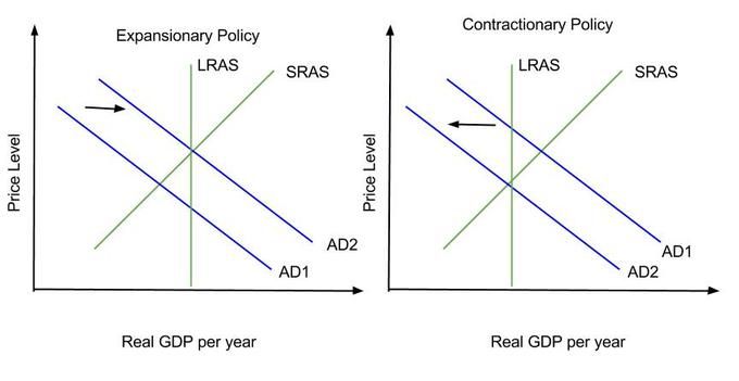
Expansionary and Contractionary Fiscal Policy: Expansionary policy shifts the AD curve to the right, while contractionary policy shifts it to the left.
It is helpful to keep in mind that aggregate demand for an economy is divided into four components: consumption, investment, government spending, and net exports. Changes in any of these components will cause the aggregate demand curve to shift.
Expansionary fiscal policy is used to kick-start the economy during a recession. It boosts aggregate demand, which in turn increases output and employment in the economy. In pursuing expansionary policy, the government increases spending, reduces taxes, or does a combination of the two. Since government spending is one of the components of aggregate demand, an increase in government spending will shift the demand curve to the right. A reduction in taxes will leave more disposable income and cause consumption and savings to increase, also shifting the aggregate demand curve to the right. An increase in government spending combined with a reduction in taxes will, unsurprisingly, also shift the AD curve to the right. The extent of the shift in the AD curve due to government spending depends on the size of the spending multiplier, while the shift in the AD curve in response to tax cuts depends on the size of the tax multiplier. If government spending exceeds tax revenues, expansionary policy will lead to a budget deficit.
A contractionary fiscal policy is implemented when there is demand-pull inflation. It can also be used to pay off unwanted debt. In pursuing contractionary fiscal policy the government can decrease its spending, raise taxes, or pursue a combination of the two. Contractionary fiscal policy shifts the AD curve to the left. If tax revenues exceed government spending, this type of policy will lead to a budget surplus.
Expansionary Versus Contractionary Fiscal Policy
When the economy is producing less than potential output, expansionary fiscal policy can be used to employ idle resources and boost output.
learning objectives
- Assess the mechanics and outcomes of fiscal policy
Counter-cyclical Fiscal Policies: Keynesian economists advocate counter-cyclical fiscal policies. This means increased spending and lower taxes during recessions and lower spending and higher taxes during economic boom times.
According to Keynesian economics, if the economy is producing less than potential output, government spending can be used to employ idle resources and boost output. Increased government spending will result in increased aggregate demand, which then increases the real GDP, resulting in an rise in prices. This is known as expansionary fiscal policy. Conversely, in times of economic expansion, the government can adopt a contractionary policy, decreasing spending, which decreases aggregate demand and the real GDP, resulting in a decrease in prices.

Highway Construction: The government can implement expansionary fiscal policy through increased spending, such as paying for the construction of new highways.
In instances of recession, government spending does not have to make up for the entire output gap. There is a multiplier effect that boosts the impact of government spending. The government could stimulate a great deal of new production with a modest expenditure increase if the people who receive this money consume most of it. This extra spending allows businesses to hire more people and pay them, which in turn allows a further increase in spending, and so on in a virtuous circle.
In addition to changes in spending, the government can also close recessionary gaps by decreasing income taxes, which increases aggregate demand and real GDP, which in turn increases prices. Conversely, to close an expansionary gap, the government would increase income taxes, which decreases aggregate demand, the real GDP, and then prices.
The effects of fiscal policy can be limited by crowding out. Crowding out occurs when government spending simply replaces private sector output instead of adding additional output to the economy. Crowding out also occurs when government spending raises interest rates, which limits investment.
Fiscal Levers: Spending and Taxation
Tax cuts have a smaller affect on aggregate demand than increased government spending.
learning objectives
- Analyze the use of changes in the tax rate as a form of fiscal policy
Spending and taxation are the two levers available to the government for setting fiscal policy. In expansionary fiscal policy, the government increases its spending, cuts taxes, or a combination of both. The increase in spending and tax cuts will increase aggregate demand, but the extent of the increase depends on the spending and tax multipliers.
The government spending multiplier is a number that indicates how much change in aggregate demand would result from a given change in spending. The government spending multiplier effect is evident when an incremental increase in spending leads to an rise in income and consumption. The tax multiplier is the magnification effect of a change in taxes on aggregate demand. The decrease in taxes has a similar effect on income and consumption as an increase in government spending.
However, the tax multiplier is smaller than the spending multiplier. This is because when the government spends money, it directly purchases something, causing the full amount of the change in expenditure to be applied to the aggregate demand. When the government cuts taxes instead, there is an increase in disposable income. Part of the disposable income will be spent, but part of it will be saved. The money that is saved does not contribute to the multiplier effect.

Spending and Saving: The tax multiplier is smaller than the government expenditure multiplier because some of the increase in disposable income that results from lower taxes is not just consumed, but saved.
The multipliers are calculated as follows:
where MPC is the marginal propensity to consume (the change in consumption divided by the change in disposable income), and MPS is the marginal propensity to save (the change in savings divided by the change in disposable income).
The government spending multiplier is always positive. In contrast, the tax multiplier is always negative. This is because there is an inverse relationship between taxes and aggregate demand. When taxes decrease, aggregate demand increases.
The multiplier effect of a tax cut can be affected by the size of the tax cut, the marginal propensity to consume, as well as the crowding out effect. The crowding out effect occurs when higher income leads to an increased demand for money, causing interest rates to rise. This leads to a reduction in investment spending, one of the four components of aggregate demand, which mitigates the increase in aggregate demand otherwise caused by lower taxes.
How Fiscal Policy Can Impact GDP
Fiscal policy impacts GDP through the fiscal multiplier.
learning objectives
- Discuss the mechanisms that allow the fiscal policy to affect GDP
Expansionary fiscal policy can impact the gross domestic product (GDP) through the fiscal multiplier. The fiscal multiplier (which is not to be confused with the monetary multiplier) is the ratio of a change in national income to the change in government spending that causes it. When this multiplier exceeds one, the enhanced effect on national income is called the multiplier effect.
The multiplier effect arises when an initial incremental amount of government spending leads to increased income and consumption, increasing income further, and hence further increasing consumption, and so on, resulting in an overall increase in national income that is greater than the initial incremental amount of spending. In other words, an initial change in aggregate demand may cause a change in aggregate output (and hence the aggregate income that it generates) that is a multiple of the initial change. The multiplier effect has been used as an argument for the efficacy of government spending or taxation relief to stimulate aggregate demand.
For example, suppose the government spends $1 million to build a plant. The money does not disappear, but rather becomes wages to builders, revenue to suppliers, etc. The builders then will have more disposable income, and consumption may rise, so that aggregate demand will also rise. Suppose further that recipients of the new spending by the builder in turn spend their new income, raising demand and possibly consumption further, and so on. The increase in the gross domestic product is the sum of the increases in net income of everyone affected. If the builder receives $1 million and pays out $800,000 to sub contractors, he has a net income of $200,000 and a corresponding increase in disposable income (the amount remaining after taxes). This process proceeds down the line through subcontractors and their employees, each experiencing an increase in disposable income to the degree the new work they perform does not displace other work they are already performing. Each participant who experiences an increase in disposable income then spends some portion of it on final (consumer) goods, according to his or her marginal propensity to consume, which causes the cycle to repeat an arbitrary number of times, limited only by the spare capacity available.

Fiscal Multiplier Example: The money spent on construction of a plant becomes wages to builders. The builders will have more disposable income, increasing their consumption and the aggregate demand.
In certain cases multiplier values of less than one have been empirically measured, suggesting that certain types of government spending crowd out private investment or consumer spending that would have otherwise taken place.
Fiscal Policy and the Multiplier
Fiscal policy can have a multiplier effect on the economy.
learning objectives
- Describe the effects of the multiplier beyond its relevance to fiscal policy
Fiscal policy can have a multiplier effect on the economy. For example, if a $100 increase in government spending causes the GDP to increase by $150, then the spending multiplier is 1.5. In addition to the spending multiplier, other types of fiscal multipliers can also be calculated, like multipliers that describe the effects of changing taxes. The size of the multiplier effect depends upon the fiscal policy.
Expansionary fiscal policy can lead to an increase in real GDP that is larger than the initial rise in aggregate spending caused by the policy. Conversely, contractionary fiscal policy can lead to a fall in real GDP that is larger than the initial reduction in aggregate spending caused by the policy.
Multiplier Effect: The multiplier effect determines the extent to which fiscal policy shifts the aggregate demand curve and impacts output.
The size of the shift of the aggregate demand curve and the change in output depend on the type of fiscal policy. The multiplier on changes in government purchases, 1/(1 – MPC), is larger than the multiplier on changes in taxes, MPC/(1 – MPC), because part of any change in taxes or transfers is absorbed by savings. In both of these equations, recall that MPC is the marginal propensity to consume.
For example, the government hands out $50 billion in the form of tax cuts. There is no direct effect on aggregate demand by government purchases of goods and services. Instead, GDP goes up only because households spend some of that $50 billion. But how much will they spend? Households will spend \(\mathrm\) (where MPC is the marginal propensity to consume). If MPC is equal to 0.6, the first-round increase in consumer spending will be \(\mathrm\). The initial rise in consumer spending will lead to a series of subsequent rounds in which the real GDP, disposable income, and consumer spending rise further.
Key Points
- The government has two levers when setting fiscal policy: it can change the levels of taxation and/or it can change its level of spending.
- There are three types of fiscal policy: neutral policy, expansionary policy,and contractionary policy.
- In expansionary fiscal policy, the government spends more money than it collects through taxes. This type of policy is used during recessions to build a foundation for strong economic growth and nudge the economy toward full employment.
- In contractionary fiscal policy, the government collects more money through taxes than it spends. This policy works best in times of economic booms. It slows the pace of strong economic growth and puts a check on inflation.
- Aggregate demand is made up of consumption, investment, government spending, and net exports. The aggregate demand curve will shift as a result of changes in any of these components.
- Expansionary policy involves an increase in government spending, a reduction in taxes, or a combination of the two. It leads to a right-ward shift in the aggregate demand curve.
- Contractionary policy involves a decrease in government spending, an increase in taxes, or a combination of the two. It leads to a left-ward shift in the aggregate demand curve.
- Keynes advocated counter-cyclical fiscal policies –implementing an expansionary fiscal policy during a recession and a contractionary policy during times of rapid economic expansion.
- In pursuing either expansionary or contractionary fiscal policy, the government has two levers – government spending and taxation levels.
- The effects of fiscal policy can be limited by crowding out.
- In expansionary policy, the extent to which government spending and tax cuts increase aggregate demand depends on spending and tax multipliers.
- The tax multiplier is smaller than the spending multiplier. This is because the entire government spending increase goes towards increasing aggregate demand, but only a portion of the increased disposable income (resulting for lower taxes) is consumed.
- The multiplier effect of a tax cut can be affected by the size of the tax cut, the marginal propensity to consume, as well as the crowding out effect.
- The fiscal multiplier is the ratio of change in national income to the change in governments spending that causes it.
- The multiplier effect occurs when an initial incremental amount of spending leads to an increase in income and consumption, which further increases income, which further increases consumption, and so on in a virtuous circle, resulting in an overall increase in the GDP.
- The multiplier effect is evident when the multiplier is greater or less than one.
- In certain cases, multiplier values of less than one have been empirically measured, suggesting that government spending can crowd out private investment or consumer spending.
- The size of the increase in GDP depends on the type of fiscal policy.
- The multiplier on changes in government spending is larger than the multiplier on changes in taxation levels.
- The taxation multiplier is smaller than the spending multiplier because part of any change in taxes is absorbed by savings.
Key Terms
- fiscal policy: Government policy that attempts to influence the direction of the economy through changes in government spending or taxes.
- multiplier: A ratio used to estimate total economic effect for a variety of economic activities.
- Tax multiplier: The change in aggregate demand caused by a change in taxation levels.
- fiscal multiplier: The ratio of a change in national income to the change in government spending that causes it.
LICENSES AND ATTRIBUTIONS
CC LICENSED CONTENT, SHARED PREVIOUSLY
- Curation and Revision. Provided by: Boundless.com. License: CC BY-SA: Attribution-ShareAlike
CC LICENSED CONTENT, SPECIFIC ATTRIBUTION
- fiscal policy. Provided by: Wiktionary. Located at: en.wiktionary.org/wiki/fiscal_policy. License: CC BY-SA: Attribution-ShareAlike
- Fiscal policy. Provided by: Wikipedia. Located at: en.Wikipedia.org/wiki/Fiscal_policy. License: CC BY-SA: Attribution-ShareAlike
- Fiscal policy. Provided by: Wikipedia. Located at: http://en.Wikipedia.org/wiki/Fiscal_policy. License: CC BY-SA: Attribution-ShareAlike
- Fiscal policy. Provided by: Wikipedia. Located at: http://en.Wikipedia.org/wiki/Fiscal_policy. License: CC BY-SA: Attribution-ShareAlike
- Bowery men waiting for bread in bread line, New York City, Bain Collection. Provided by: Wikimedia. Located at: commons.wikimedia.org/wiki/F. Collection.jpg. License: Public Domain: No Known Copyright
- fiscal policy. Provided by: Wiktionary. Located at: http://en.wiktionary.org/wiki/fiscal_policy. License: CC BY-SA: Attribution-ShareAlike
- UNIT 3 National Income and Price Determination. Provided by: mreape Wikispace. Located at: mreape.wikispaces.com/UNIT+3+. +Determination. License: CC BY-SA: Attribution-ShareAlike
- Fiscal Policy. Provided by: mchenry Wikispace. Located at: mchenry.wikispaces.com/Fiscal+Policy. License: CC BY-SA: Attribution-ShareAlike
- UNIT 3 National Income and Price Determination. Provided by: mreape Wikispace. Located at: mreape.wikispaces.com/UNIT+3+. +Determination. License: CC BY-SA: Attribution-ShareAlike
- Bowery men waiting for bread in bread line, New York City, Bain Collection. Provided by: Wikimedia. Located at: commons.wikimedia.org/wiki/F. Collection.jpg. License: Public Domain: No Known Copyright
- Contractionary and expansionary fiscal policy. Provided by: Wikimedia. Located at: commons.wikimedia.org/wiki/F. cal_policy.jpg. License: CC BY-SA: Attribution-ShareAlike
- Discretionary and Automatic Fiscal Policy. Provided by: econ101-powers Wikispace. Located at: econ101-powers.wikispaces.com. +Fiscal+Policy. License: CC BY-SA: Attribution-ShareAlike
- Discretionary and Automatic Fiscal Policy. Provided by: econ101-powers Wikispace. Located at: econ101-powers.wikispaces.com. +Fiscal+Policy. License: CC BY-SA: Attribution-ShareAlike
- Macroeconomics. Provided by: Wikipedia. Located at: en.Wikipedia.org/wiki/Macroeconomics. License: CC BY-SA: Attribution-ShareAlike
- Fiscal Policy, Deficit, and Surplus. Provided by: econ101-powers-sectionc Wikispace. Located at: econ101-powers-sectionc.wikis. t,+and+Surplus. License: CC BY-SA: Attribution-ShareAlike
- Keynesian economics. Provided by: Wikipedia. Located at: en.Wikipedia.org/wiki/Keynesi. _fiscal_policy. License: CC BY-SA: Attribution-ShareAlike
- Keynesian economics. Provided by: Wikipedia. Located at: en.Wikipedia.org/wiki/Keynesi. _fiscal_policy. License: CC BY-SA: Attribution-ShareAlike
- multiplier. Provided by: Wiktionary. Located at: en.wiktionary.org/wiki/multiplier. License: CC BY-SA: Attribution-ShareAlike
- Bowery men waiting for bread in bread line, New York City, Bain Collection. Provided by: Wikimedia. Located at: commons.wikimedia.org/wiki/F. Collection.jpg. License: Public Domain: No Known Copyright
- Contractionary and expansionary fiscal policy. Provided by: Wikimedia. Located at: commons.wikimedia.org/wiki/F. cal_policy.jpg. License: CC BY-SA: Attribution-ShareAlike
- All sizes | East Fork Bitterroot Road Recovery Act Project | Flickr - Photo Sharing!. Provided by: Flickr. Located at: www.flickr.com/photos/fsnorth. n/photostream/. License: CC BY: Attribution
- Contractionary and expansionary fiscal policy. Provided by: Wikimedia. Located at: commons.wikimedia.org/wiki/F. cal_policy.jpg. License: CC BY-SA: Attribution-ShareAlike
- Detail. Provided by: hfecon Wikispace. Located at: hfecon.wikispaces.com/file/de. nswer+Key.docx. License: CC BY-SA: Attribution-ShareAlike
- Detail. Provided by: hfecon Wikispace. Located at: hfecon.wikispaces.com/file/de. nswer+Key.docx. License: CC BY-SA: Attribution-ShareAlike
- Unit Three. Provided by: moeller Wikispace. Located at: moeller.wikispaces.com/Unit+Three. License: CC BY-SA: Attribution-ShareAlike
- CFA Session 6. Provided by: jiryih Wikispace. Located at: jiryih.wikispaces.com/CFA+Session+6. License: CC BY-SA: Attribution-ShareAlike
- Boundless. Provided by: Boundless Learning. Located at: www.boundless.com//economics/. tax-multiplier. License: CC BY-SA: Attribution-ShareAlike
- Bowery men waiting for bread in bread line, New York City, Bain Collection. Provided by: Wikimedia. Located at: commons.wikimedia.org/wiki/F. Collection.jpg. License: Public Domain: No Known Copyright
- Contractionary and expansionary fiscal policy. Provided by: Wikimedia. Located at: commons.wikimedia.org/wiki/F. cal_policy.jpg. License: CC BY-SA: Attribution-ShareAlike
- All sizes | East Fork Bitterroot Road Recovery Act Project | Flickr - Photo Sharing!. Provided by: Flickr. Located at: www.flickr.com/photos/fsnorth. n/photostream/. License: CC BY: Attribution
- Contractionary and expansionary fiscal policy. Provided by: Wikimedia. Located at: commons.wikimedia.org/wiki/F. cal_policy.jpg. License: CC BY-SA: Attribution-ShareAlike
- 1970sgrocerystore. Provided by: Wikimedia. Located at: commons.wikimedia.org/wiki/Fi. ocerystore.jpg. License: CC BY: Attribution
- Fiscal multiplier. Provided by: Wikipedia. Located at: en.Wikipedia.org/wiki/Fiscal_multiplier. License: CC BY-SA: Attribution-ShareAlike
- fiscal multiplier. Provided by: Wikipedia. Located at: en.Wikipedia.org/wiki/fiscal%20multiplier. License: CC BY-SA: Attribution-ShareAlike
- Bowery men waiting for bread in bread line, New York City, Bain Collection. Provided by: Wikimedia. Located at: https://commons.wikimedia.org/wiki/F. Collection.jpg. License: Public Domain: No Known Copyright
- Contractionary and expansionary fiscal policy. Provided by: Wikimedia. Located at: commons.wikimedia.org/wiki/F. cal_policy.jpg. License: CC BY-SA: Attribution-ShareAlike
- All sizes | East Fork Bitterroot Road Recovery Act Project | Flickr - Photo Sharing!. Provided by: Flickr. Located at: www.flickr.com/photos/fsnorth. n/photostream/. License: CC BY: Attribution
- Contractionary and expansionary fiscal policy. Provided by: Wikimedia. Located at: commons.wikimedia.org/wiki/F. cal_policy.jpg. License: CC BY-SA: Attribution-ShareAlike
- 1970sgrocerystore. Provided by: Wikimedia. Located at: commons.wikimedia.org/wiki/Fi. ocerystore.jpg. License: CC BY: Attribution
- Construction Workers. Provided by: Wikimedia. Located at: commons.wikimedia.org/wiki/Fi. on_Workers.jpg. License: CC BY: Attribution
- Detail. Provided by: nrapmacro Wikispace. Located at: nrapmacro.wikispaces.com/file. l/Module21.ppt. License: CC BY-SA: Attribution-ShareAlike
- Detail. Provided by: nrapmacro Wikispace. Located at: nrapmacro.wikispaces.com/file. l/Module21.ppt. License: CC BY-SA: Attribution-ShareAlike
- Multiplier (economics). Provided by: Wikipedia. Located at: en.Wikipedia.org/wiki/Multiplier_(economics). License: CC BY-SA: Attribution-ShareAlike
- fiscal multiplier. Provided by: Wikipedia. Located at: en.Wikipedia.org/wiki/fiscal%20multiplier. License: CC BY-SA: Attribution-ShareAlike
- Bowery men waiting for bread in bread line, New York City, Bain Collection. Provided by: Wikimedia. Located at: https://commons.wikimedia.org/wiki/F. Collection.jpg. License: Public Domain: No Known Copyright
- Contractionary and expansionary fiscal policy. Provided by: Wikimedia. Located at: commons.wikimedia.org/wiki/F. cal_policy.jpg. License: CC BY-SA: Attribution-ShareAlike
- All sizes | East Fork Bitterroot Road Recovery Act Project | Flickr - Photo Sharing!. Provided by: Flickr. Located at: www.flickr.com/photos/fsnorth. n/photostream/. License: CC BY: Attribution
- Contractionary and expansionary fiscal policy. Provided by: Wikimedia. Located at: commons.wikimedia.org/wiki/F. cal_policy.jpg. License: CC BY-SA: Attribution-ShareAlike
- 1970sgrocerystore. Provided by: Wikimedia. Located at: commons.wikimedia.org/wiki/Fi. ocerystore.jpg. License: CC BY: Attribution
- Construction Workers. Provided by: Wikimedia. Located at: commons.wikimedia.org/wiki/Fi. on_Workers.jpg. License: CC BY: Attribution
- Contractionary and expansionary fiscal policy. Provided by: Wikimedia. Located at: commons.wikimedia.org/wiki/File:Contractionary_and_expansionary_fiscal_policy.jpg. License: CC BY-SA: Attribution-ShareAlike
This page titled 26.1: Introduction to Fiscal Policy is shared under a CC BY-SA 4.0 license and was authored, remixed, and/or curated by Boundless.
- Back to top
- 26: Fiscal Policy
- 26.2: Evaluating Fiscal Policy
- Was this article helpful?
- Yes
- No
